What type of analyst and intellectual would it be without a proper notebook and records about his petty successes in data science or data engineering? Although there are many such interesting and successful people without need to take notes, I found that taking notes about the progress in work in somehow satisfying and good for thinking about next development steps.

In this series of posts, I will try to share my notes about the development of a dashboard for climate data. I will share the code snippets, data sources and thoughts behind the development of the project. I hope that it will be useful for someone who is interested in the topic and wants to learn more about it.

Intention of the project

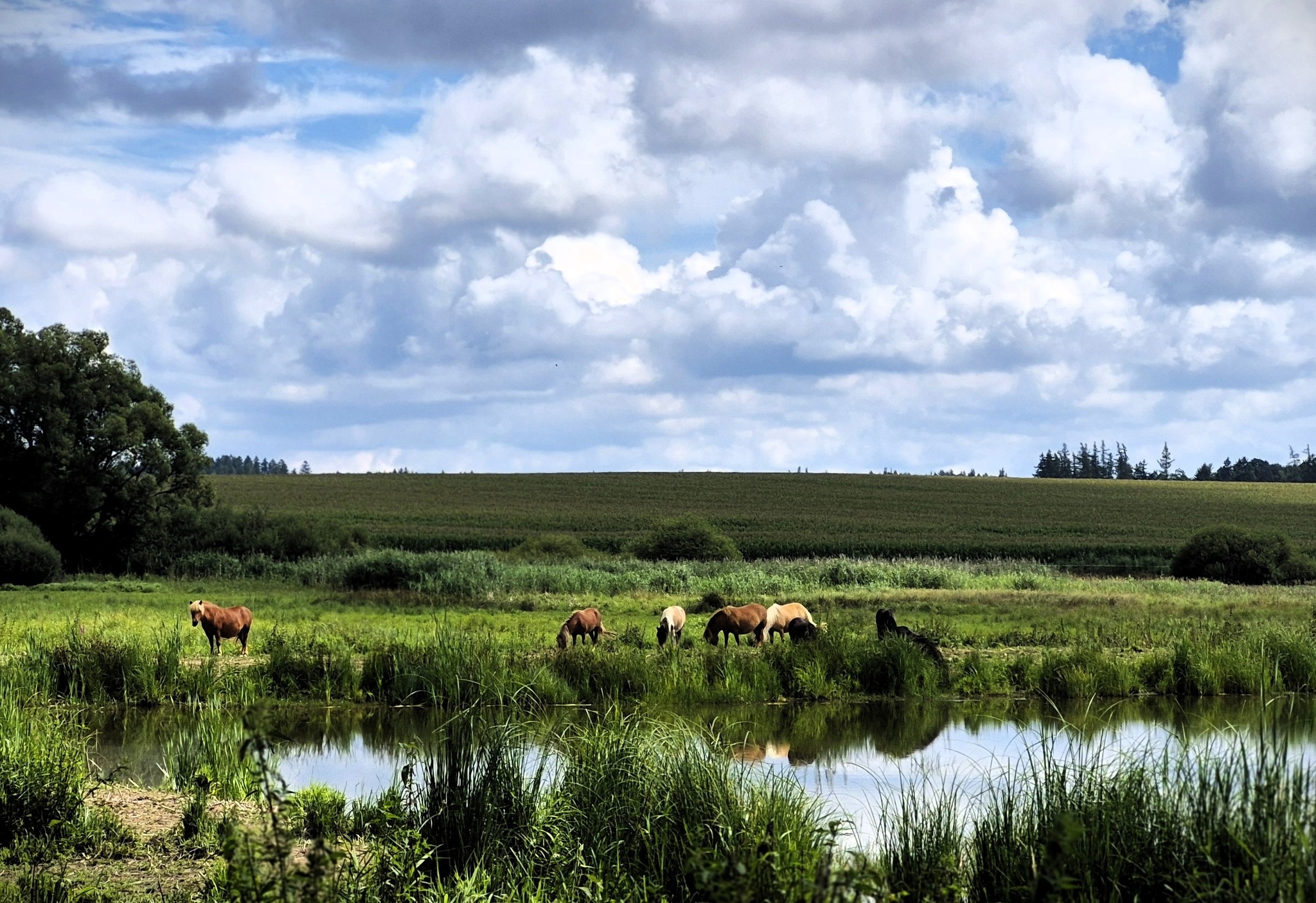
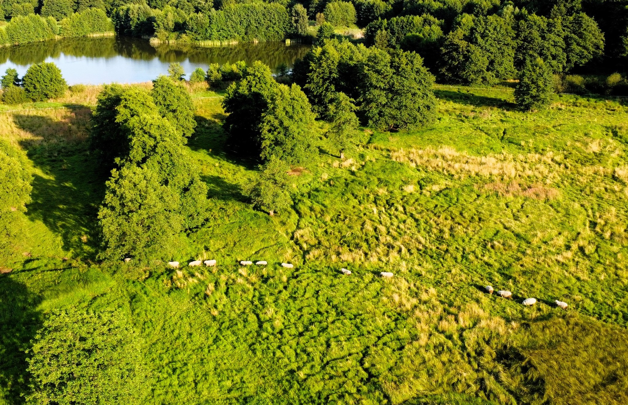
You see, I am an agroclimatic data analyst and improving skills in data engineering is quite important for me. There is another reason for such work – my family own summer house in the countryside and one part of the affiliated land is located in the area were lake was located. The lake leaked and now there is a wetland. The entire area is now protected due to the presence of rare species of birds, amphibians and plants.

I am interested in the changes in the area and how they are related to climate change. The desired dashboard will allow me to visualise the data and see the trends in the area, which can be crucial for the future of the area and its inhabitants.

Also, I am interested in agricultural fields and in their productivity in the vicinity of the Nature park. I want to see how the weather patterns are changing and how they are affecting the crops.

Finally, I want to share the dashboard with my family and friends, so they can also see the changes in the area and understand the importance of climate change. So, that’s a lot of plans for the project! Let’s not loose the time and start with the data access!

Software and tools

Necessary software and tools for the project are:

• Python 3.11 or higher (especially zarr>3)
• Any code editor (e.g. VSCode, PyCharm, Jupyter Notebook)
• Any software for reading CSV or XLSX files (e.g. Excel, LibreOffice)

My setup is based on VS Code and Jupyter Notebook with a virtual environment for Python. The virtual environment is recommended for the project, because it allows to keep the dependencies and packages organised and separated from other projects. However, you can easily run the code in a basic Python environment if you don’t have other projects with conflicting dependencies.

Requested datasets

There are many interesting data sources for climate data from various agencies and organisations. There are datasets from NASA, NOAA, ECMWF, Copernicus and many others, and they can differ from each other in terms of spatial and temporal resolution, variables, format and accessibility. It would be quite complicated to describe all characteristics of every dataset, so let’s skip the details (topic for future posts) and choose two types of datasets for our work. They are quite easily accessible, popular enough and serve well for the planned dashboard.

We will be using weather data for a single point and for that we don’t need to work with spatial formats using geospatial libraries or spatial file formats like netcdf. Our goal is to create table or a dataframe with time series of weather variables.

So, the first dataset will be the NASA POWER dataset, which is very easily accessible via API. It has decent spatial and temporal resolution, as well as temporal coverage. The parameters are as follows:

The second dataset will be the ERA5 dataset provided by ECMWF, and originally accessible via Copernicus Climate Data Store. However, there is a new service the Earth Data Hub, which allows access to the data via a simple API, without the necessity to download netCDF files. The dataset has nice spatial and temporal resolution, with high temporal coverage. The characteristics of the dataset are as follows:

*Native resolution is 9 km – that’s the resolution of the model’s calculations.

Requested datasets

Let’s very quickly review the variables that will be requested from the NASA POWER and ERA5 catalogues.

The NASA POWER dataset has many variables to choose from (there will be a script later in the post to see all available variables), but we will be using the following ones:

The final dataset should include the following variables:

The Earth Data Hub provides access to the ERA5 dataset, which has a limited number of variables available from its catalogue, but still a sufficient selection for our purposes. The variables are as follows:

Python code

Let’s start with importing the necessary Python libraries for the first part of the project:

import xarray as xr # for accessing the Earth Data Hub
import requests # for acessing the NASA POWER database
import pandas as pd # for general data wrangling
import numpy as np # for minor task - labeling NaN values
import datetime as dt # for standard datetime formats

from dask.diagnostics import ProgressBar # to see data download progress 

import xarray as xr # for accessing the Earth Data Hub
import requests # for acessing the NASA POWER database
import pandas as pd # for general data wrangling
import numpy as np # for minor task - labeling NaN values
import datetime as dt # for standard datetime formats

from dask.diagnostics import ProgressBar # to see data download progress 

Choosing the location from which data will be downloaded is the first step in the project. I will be using the coordinates of the point of interest, which is located in the area of the wetland. You can easily copy them from Google Maps or Mapy.com. My coordinates are as follows:

# location coordinates
point_lat, point_lon = 49.73206632355159, 15.553702007963855

# location coordinates
point_lat, point_lon = 49.73206632355159, 15.553702007963855

NASA POWER dataset

We will start with the NASA POWER and the first step is optional. Let’s see what variables are accessible via API. The following function will return the dataframe (table) with all variables and their metadata (definitions, source, name or code).

def show_variables():
    url = "https://power.larc.nasa.gov/api/system/manager/parameters"
    params = {
        "community": "AG",
        "temporal": "daily"
    }

    r = requests.get(url, params=params)
    r.raise_for_status()
    data = r.json()

    rows = []
    for code, meta in data.items():
        row = {"code": code}

        if isinstance(meta, dict):
            for k, v in meta.items():
                if not isinstance(v, (dict, list)):
                    row[k] = v
        rows.append(row)

    df = pd.DataFrame(rows)
    return df

def show_variables():
    url = "https://power.larc.nasa.gov/api/system/manager/parameters"
    params = {
        "community": "AG",
        "temporal": "daily"
    }

    r = requests.get(url, params=params)
    r.raise_for_status()
    data = r.json()

    rows = []
    for code, meta in data.items():
        row = {"code": code}

        if isinstance(meta, dict):
            for k, v in meta.items():
                if not isinstance(v, (dict, list)):
                    row[k] = v
        rows.append(row)

    df = pd.DataFrame(rows)
    return df

After you run the function, you can continue with the selected variables and their codes for the API request. Let’s create a list of variables based on the table above:

power_variables = ["TOA_SW_DWN", "ALLSKY_SFC_SW_DWN", "T2M", "T2M_MIN",
                    "T2M_MAX", "T2MDEW", "WS2M", "PRECTOTCORR", "RH2M"]

power_variables = ["TOA_SW_DWN", "ALLSKY_SFC_SW_DWN", "T2M", "T2M_MIN",
                    "T2M_MAX", "T2MDEW", "WS2M", "PRECTOTCORR", "RH2M"]

Now we can create the function to download the data from NASA POWER API. The following function, again using the request library, will send the request and return the data in JSON format.

def Query_NASA_POWER(latitude, longitude, power_variables):
        """
        Query the NASA POWER server for specific location
        """

        start_date = dt.date(1981,1,1)
        end_date = dt.date.today()

        # build URL for retrieving data, using new NASA POWER api
        server_url = "https://power.larc.nasa.gov/api/temporal/daily/point"
        payload = {"request": "execute",
                   "parameters": ",".join(power_variables),
                   "latitude": latitude,
                   "longitude": longitude,
                   "start": start_date.strftime("%Y%m%d"),
                   "end": end_date.strftime("%Y%m%d"),
                   "community": "AG",
                   "format": "JSON",
                   "user": "LT"
                   }
        print("Starting retrieval from NASA Power")
        req = requests.get(server_url, params=payload)

        HTTP_OK = 200

        if req.status_code != HTTP_OK:
            print("Failed retrieving POWER data, server returned HTTP " +
                   "code: %i on following URL %s") % (req.status_code, req.url)

        print("Successfully downloaded climate data from NASA POWER server")
        return req.json()

def Query_NASA_POWER(latitude, longitude, power_variables):
        """
        Query the NASA POWER server for specific location
        """

        start_date = dt.date(1981,1,1)
        end_date = dt.date.today()

        # build URL for retrieving data, using new NASA POWER api
        server_url = "https://power.larc.nasa.gov/api/temporal/daily/point"
        payload = {"request": "execute",
                   "parameters": ",".join(power_variables),
                   "latitude": latitude,
                   "longitude": longitude,
                   "start": start_date.strftime("%Y%m%d"),
                   "end": end_date.strftime("%Y%m%d"),
                   "community": "AG",
                   "format": "JSON",
                   "user": "LT"
                   }
        print("Starting retrieval from NASA Power")
        req = requests.get(server_url, params=payload)

        HTTP_OK = 200

        if req.status_code != HTTP_OK:
            print("Failed retrieving POWER data, server returned HTTP " +
                   "code: %i on following URL %s") % (req.status_code, req.url)

        print("Successfully downloaded climate data from NASA POWER server")
        return req.json()

So we can run it with our coordinates and selected variables and assign the result to the variable:

JSON_data = Query_NASA_POWER(point_lat, point_lon, power_variables)

JSON_data = Query_NASA_POWER(point_lat, point_lon, power_variables)

Let’s check the metadata of JSON response. We can see that there is some information about elevation, fill value for missing data and sources of data. We can extract this information and print it out:

description = [JSON_data["header"]["title"]]
elevation = float(JSON_data["geometry"]["coordinates"][2])
fill_value = float(JSON_data["header"]["fill_value"])
api_info = JSON_data["header"]["sources"]
print(description, elevation, fill_value, api_info)

description = [JSON_data["header"]["title"]]
elevation = float(JSON_data["geometry"]["coordinates"][2])
fill_value = float(JSON_data["header"]["fill_value"])
api_info = JSON_data["header"]["sources"]
print(description, elevation, fill_value, api_info)

Now it is time to change the data from JSON format to something more cosy for data analysis – DataFrame. The following function handles the so called data wrangling. It will take variables and their values, change the fill values to NaN and drop the rows with missing values. Finally, it will return the DataFrame with clean data ready for analysis. Also, it will print the length of the DataFrame before and after dropping the missing values, so we can see that there are some missing values. It is important for future decision about interpolation

def POWER_data_to_DF(JSON_data, power_variables):
    print("Wrangling the data from JSON file to Dataframe")        
    Nan = float(JSON_data["header"]["fill_value"])

    power_data_df = {}
    # Building the series and then a DataFrame
    for variable in power_variables:
        series = pd.Series(JSON_data["properties"]["parameter"][variable])
        series[series == Nan] = np.nan
        power_data_df[variable] = series
    power_data_df = pd.DataFrame(power_data_df)    
    power_data_df["time"] = pd.to_datetime(power_data_df.index, format="%Y%m%d")
    print("Length of dataframe", len(power_data_df))  

    # Locating missing values (NaN)
    print("Length of any NaN values", len(power_data_df[power_data_df.isna().any(axis=1)]))
    missing_values = power_data_df.isnull().any(axis=1)
    # Dropping missing values
    power_data_df = power_data_df[~missing_values]
    print("Length of dataframe after dropping NaN values", len(power_data_df)) 
    return power_data_df

power_data_df = POWER_data_to_DF(JSON_data, power_variables)

def POWER_data_to_DF(JSON_data, power_variables):
    print("Wrangling the data from JSON file to Dataframe")        
    Nan = float(JSON_data["header"]["fill_value"])

    power_data_df = {}
    # Building the series and then a DataFrame
    for variable in power_variables:
        series = pd.Series(JSON_data["properties"]["parameter"][variable])
        series[series == Nan] = np.nan
        power_data_df[variable] = series
    power_data_df = pd.DataFrame(power_data_df)    
    power_data_df["time"] = pd.to_datetime(power_data_df.index, format="%Y%m%d")
    print("Length of dataframe", len(power_data_df))  

    # Locating missing values (NaN)
    print("Length of any NaN values", len(power_data_df[power_data_df.isna().any(axis=1)]))
    missing_values = power_data_df.isnull().any(axis=1)
    # Dropping missing values
    power_data_df = power_data_df[~missing_values]
    print("Length of dataframe after dropping NaN values", len(power_data_df)) 
    return power_data_df

power_data_df = POWER_data_to_DF(JSON_data, power_variables)

The major final step deals with renaming the variables and converting the units of some variables to make data more standardized and ready for use in dashboard. For converting the units, we will use very useful lambda function inteded for simple operations. The function will convert the solar radiation from MJ/m²/day to J/m²/day. The remaining variables will just be renamed to something more intuitive and short.

MJ_to_J = lambda x: x * 1e6

def Rename_convert_variables(dataset):
    # Convert data to a dataframe with PCSE/Agroclimatic compatible iput names and units
    df_final = pd.DataFrame({"TMAX": dataset['T2M_MAX'],
                            "TMIN": dataset['T2M_MIN'],
                            "TEMP": dataset['T2M'],
                            "IRRAD": dataset['ALLSKY_SFC_SW_DWN'].apply(MJ_to_J),
                            "TOA_IRRAD" : dataset['TOA_SW_DWN'].apply(MJ_to_J),
                            "RAIN": dataset['PRECTOTCORR'],
                            "WIND": dataset['WS2M'],
                            "TEMPDEW": dataset['T2MDEW'],
                            "RH": dataset['RH2M'],
                            "DAY": pd.to_datetime(dataset.index, format="%Y%m%d"),
                            "LAT": point_lat,
                            "LON": point_lon,
                            "Power_ELEV": elevation})
    df_final = df_final.reset_index(drop = True)            
    return df_final
df_final = Rename_convert_variables(power_data_df)

MJ_to_J = lambda x: x * 1e6

def Rename_convert_variables(dataset):
    # Convert data to a dataframe with PCSE/Agroclimatic compatible iput names and units
    df_final = pd.DataFrame({"TMAX": dataset['T2M_MAX'],
                            "TMIN": dataset['T2M_MIN'],
                            "TEMP": dataset['T2M'],
                            "IRRAD": dataset['ALLSKY_SFC_SW_DWN'].apply(MJ_to_J),
                            "TOA_IRRAD" : dataset['TOA_SW_DWN'].apply(MJ_to_J),
                            "RAIN": dataset['PRECTOTCORR'],
                            "WIND": dataset['WS2M'],
                            "TEMPDEW": dataset['T2MDEW'],
                            "RH": dataset['RH2M'],
                            "DAY": pd.to_datetime(dataset.index, format="%Y%m%d"),
                            "LAT": point_lat,
                            "LON": point_lon,
                            "Power_ELEV": elevation})
    df_final = df_final.reset_index(drop = True)            
    return df_final
df_final = Rename_convert_variables(power_data_df)

The final dataset is now ready to use for different purposes. We can continue in python with data analysis and other operations or simply export it to csv or excel file and use it in other software. The following line of code will export the data to a CSV file:

# export to csv
df_final.to_csv("NASA_POWER_data.csv", index=False)
# export to excel
df_final.to_excel("NASA_POWER_data.xlsx", index=False)

# export to csv
df_final.to_csv("NASA_POWER_data.csv", index=False)
# export to excel
df_final.to_excel("NASA_POWER_data.xlsx", index=False)

Earth Data Hub – ERA5 dataset

Beginning of the data access from the Earth Data Hub is little bit more complicated than in previous case, but it is still quite straightforward. The first step is going to Getting Started and going through the steps to setup your credentials for authenticated data access. You will also need some additional libraries used by the Xarray, which we already imported in the beginning of the post. You can install them using pip:

pip install xarray zarr dask aiohttp

pip install xarray zarr dask aiohttp

After that, you can easily define the function to access the server and to download the data for our point of interest as well as for the selected time period. I’ve chosen the time period from 1950-01-01 to the last closed month, but shorter period from 1979-01-01 should be considered as well, because of the quality of data before 1979 (No satellite data before 1979; let’s discussed it in the future posts). The function will return the DataFrame similar to the one from NASA POWER.

def earthdatahub_access(start, end, longitude, latitude):
    ds = xr.open_dataset(
        "https://data.earthdatahub.destine.eu/era5/era5-land-daily-utc-v1.zarr",
        storage_options={"client_kwargs":{"trust_env":True}},
        chunks={},
        engine="zarr"
        )
    ds_sel = ds.sel(valid_time=slice(start, end))
    pnt = ds_sel.sel(longitude=longitude, latitude=latitude, method="nearest")
    with ProgressBar():
        pnt_df = pnt.to_dataframe().reset_index(drop=False)
    return pnt_df

# start = "1950-01-01", end = dt.date.today() or any other date - "1970-06-07"
start = "1950-01-01"
end = dt.date.today()

pnt_df =  earthdatahub_access(start, end, point_lon, point_lat)

def earthdatahub_access(start, end, longitude, latitude):
    ds = xr.open_dataset(
        "https://data.earthdatahub.destine.eu/era5/era5-land-daily-utc-v1.zarr",
        storage_options={"client_kwargs":{"trust_env":True}},
        chunks={},
        engine="zarr"
        )
    ds_sel = ds.sel(valid_time=slice(start, end))
    pnt = ds_sel.sel(longitude=longitude, latitude=latitude, method="nearest")
    with ProgressBar():
        pnt_df = pnt.to_dataframe().reset_index(drop=False)
    return pnt_df

# start = "1950-01-01", end = dt.date.today() or any other date - "1970-06-07"
start = "1950-01-01"
end = dt.date.today()

pnt_df =  earthdatahub_access(start, end, point_lon, point_lat)

If you would like to see what is going on during the data download and understand the xarray and dask operations, extract the single lines from the function and run them one by one with print or display (from IPython.display import display) of the itermediate results.

Finally, we can do the same as in previous case – rename the variables and convert the units. The following function will do that for us. The conversion of temperature from Kelvin to Celsius and precipitation from m to mm is done by lambda function. As you can see, there some variables that quite weird. Namely, the U10 and V10. We will look at them closely in the future post, but for now we can just keep them as they are. The final dataset will be exported to CSV and an Excel file, as in the previous case.

Kelvin_to_C = lambda x: x - 273.15
m_to_mm = lambda x: x * 1e3

def Rename_convert_variables2(dataset):
    # Convert data to a dataframe with Agroclimatic compatible iput names and units
    df_final = pd.DataFrame({"TOT EVAP": dataset['e'].apply(m_to_mm),
                            "PE": dataset['pev'].apply(m_to_mm),
                            "TEMP": dataset['t2m'].apply(Kelvin_to_C),
                            "TEMPDEW": dataset['d2m'].apply(Kelvin_to_C),
                            "RUNOFF": dataset['ro'].apply(m_to_mm),
                            "SURF_PRESS" : dataset['sp'],
                            "RAIN": dataset['tp'].apply(m_to_mm),
                            "U10": dataset['u10'],
                            "V10": dataset['v10'],
                            "Surface net short-wave radiation": dataset['ssr'],
                            "Surface short-wave radiation downwards": dataset['ssrd'],
                            "Surface net long-wave (thermal) radiation": dataset['str'],
                            "VOL SOIL 1": dataset['swvl1'],
                            "VOL SOIL 2": dataset['swvl2'],
                            "DAY": dataset['valid_time'],
                            "LAT": dataset['latitude'],
                            "LON": dataset['longitude']})
    df_final = df_final.reset_index(drop = True)            
    return df_final
df_final_2 = Rename_convert_variables2(pnt_df)

# export to csv
df_final_2.to_csv("NASA_POWER_data.csv", index=False)
# export to excel
df_final_2.to_excel("NASA_POWER_data.xlsx", index=False)

Kelvin_to_C = lambda x: x - 273.15
m_to_mm = lambda x: x * 1e3

def Rename_convert_variables2(dataset):
    # Convert data to a dataframe with Agroclimatic compatible iput names and units
    df_final = pd.DataFrame({"TOT EVAP": dataset['e'].apply(m_to_mm),
                            "PE": dataset['pev'].apply(m_to_mm),
                            "TEMP": dataset['t2m'].apply(Kelvin_to_C),
                            "TEMPDEW": dataset['d2m'].apply(Kelvin_to_C),
                            "RUNOFF": dataset['ro'].apply(m_to_mm),
                            "SURF_PRESS" : dataset['sp'],
                            "RAIN": dataset['tp'].apply(m_to_mm),
                            "U10": dataset['u10'],
                            "V10": dataset['v10'],
                            "Surface net short-wave radiation": dataset['ssr'],
                            "Surface short-wave radiation downwards": dataset['ssrd'],
                            "Surface net long-wave (thermal) radiation": dataset['str'],
                            "VOL SOIL 1": dataset['swvl1'],
                            "VOL SOIL 2": dataset['swvl2'],
                            "DAY": dataset['valid_time'],
                            "LAT": dataset['latitude'],
                            "LON": dataset['longitude']})
    df_final = df_final.reset_index(drop = True)            
    return df_final
df_final_2 = Rename_convert_variables2(pnt_df)

# export to csv
df_final_2.to_csv("NASA_POWER_data.csv", index=False)
# export to excel
df_final_2.to_excel("NASA_POWER_data.xlsx", index=False)

And that’s it – we’ve covered quite a lot! ⚙️🌱💡

It turned out to be a longer post in the end and lot of new information, but now you can access climate data for your own point of interest and maybe start with some basic data analysis and visualization. Hopefully it will lead to some groundbreaking insights about climate change in your area.

In the next part of the project, we will look at the data, compare the two datasets, maybe find some interesting patterns and talk little bit about the characteristics of the datasets and their differences. Also, we will look at these wind variables and how to transform them to something more interesting for us. Stay tuned! 🚀